Forest Canopy Change (FCC)
FCC product maps the drop or regrowth in canopy densities that have occured within a period, either as a difference from the consequent years or a difference from a comparison (baseline) period i.e 2016. The computation of the difference highlights areas that have since experienced canopy disturbance, regrowth or are stable. The computation is based on a simple image difference between the comparison period and analysis period. To compute FCC, two approaches are majorly employed, including.
Changes based on the Reference year i.e 2016 (Reference Product).
Changes based on the difference between the consequent year (Annual Product).
Reference Product
Reference Products are achieved after computing the difference between the compasrison yearbaseline year (2016), and the other consequent years i.e 2017, 2018, 2019 & 2020. This product detects the deforestation that occurs in comparison to the baseline year which is 2016. The output and statistics assumes the forest zones are instant forest. Classifying the forest canopy densities, makes it possible to monitor forest disturbances every year, in each forest of interest.
Annual Product
The changes are computed in comparison to the consequent years. In monitoring the forest regrowth between two years, this product can be applied. The changes are generated after computing the difference between the forest canopy densities from 2016 - 2020 The products available are in the TroFMIS 2016 - 2017, 2017 - 2018, 2018 - 2019 & 2019 - 2020, and the updating of newer products will be done once the satellite images for the entire year are available.
The figure below shows the summary of computing the forest changes.
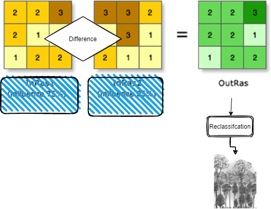
Fig. 2 Forest Canopy Changes computation.
Computing the FCC products in Google Earth Engine
The code provided in the Forest Canopy Density section, provides a multi products as outputs, and this include both the * Forest Canopy Densities and * Forest Canopy Changes both annual and Reference product.
The description of the screen shot below from the main code highlights how the Changes are generated.
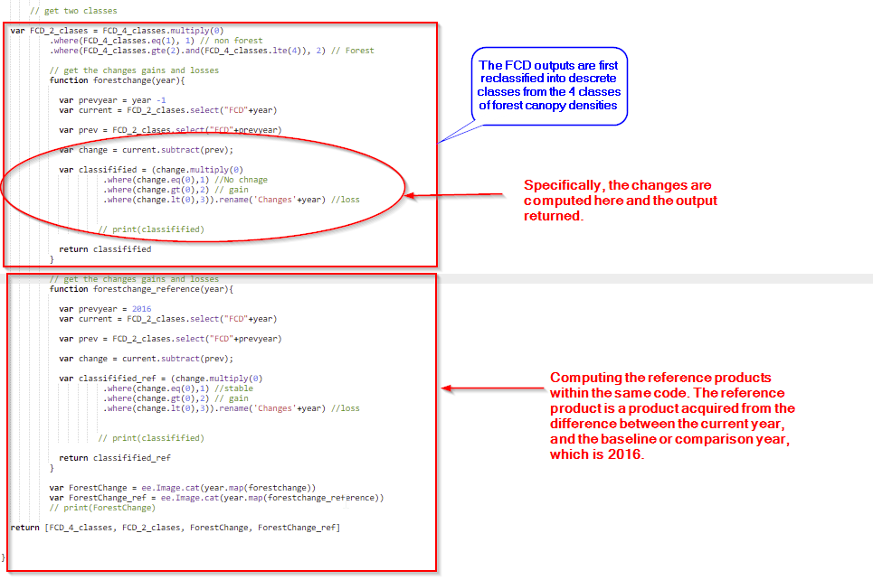
The code to generate the multi prouct is also encompassed below.
Step 1. Example:
var FCD_2_clases = FCD_4_classes.multiply(0)
           .where(FCD_4_classes.eq(1), 1) // non forest
           .where(FCD_4_classes.gte(2).and(FCD_4_classes.lte(4)), 2) // Forest

           // get the changes gains and losses
           function forestchange(year){

             var prevyear = year -1
             var current = FCD_2_clases.select("FCD"+year)

             var prev = FCD_2_clases.select("FCD"+prevyear)

             var change = current.subtract(prev);

             var classifified = (change.multiply(0)
                      .where(change.eq(0),1) //No chnage
                      .where(change.gt(0),2) // gain
                      .where(change.lt(0),3)).rename('Changes'+year) //loss


                     // print(classifified)

             return classifified
           }

           // get the changes gains and losses
           function forestchange_reference(year){

             var prevyear = 2016
             var current = FCD_2_clases.select("FCD"+year)

             var prev = FCD_2_clases.select("FCD"+prevyear)

             var change = current.subtract(prev);

             var classifified_ref = (change.multiply(0)
                      .where(change.eq(0),1) //stable
                      .where(change.gt(0),2) // gain
                      .where(change.lt(0),3)).rename('Changes'+year) //loss


                     // print(classifified)

             return classifified_ref
           }

           var ForestChange = ee.Image.cat(year.map(forestchange))
           var ForestChange_ref = ee.Image.cat(year.map(forestchange_reference))
           // print(ForestChange)

   return [FCD_4_classes, FCD_2_clases, ForestChange, ForestChange_ref]
Just like the FCD products, the forest change products are exported in drive, and the finall geotiff files will require mosaicking. The Forest Change products come as a multiband raster, and will also be loaded as a multi band raster in the database. The use of R code is also employed in mosaicking the multiband rasters and saving them in a folder before updating in the database.
library(raster)
library(sp)
library(ggplot2)


      setwd("H:/1.FORESTT/Sentinel_2/mosaic")
      getwd()

      year<-"2019"
      country<-"Uganda"
      fn<- paste('FCD_',country,year,'Sentinel_2_mos.tif',sep="")

      my_dirs<- paste("G:/My Drive/TROFMIS_UgandaSentinel_changes",year, sep="")


      all_text_files <- list.files(my_dirs, pattern = "\\.tif$", full.names = TRUE)

      print(length(all_text_files))

      for (file in all_text_files){

        print(file)
      }

      print(length(all_text_files))

      r1<-stack(all_text_files[1])
      r2<-stack(all_text_files[2])
      r3<-stack(all_text_files[3])
      r4<-stack(all_text_files[4])
      r5<-stack(all_text_files[5])
      r6<-stack(all_text_files[6])
      print(r19)

      rmoz<- mosaic(r1,r2,r3,r4,r5,r6
                    ,fun = mean, tolerance=0.05, filename = 'change.tif')
      plot(rmoz)
To use R in mosaicking, it is vital that the working directory is set prior to computation. This is to allow the files to be read and writtenly seamlessly, as well as to avoid errors that might arise.
Forest Change Encoding
Forest Changes come in a multi band format, whereby, each product has 3 bands encorded as follows.
Band Value |
Class |
Max |
|---|---|---|
1 |
Stable |
1 |
2 |
Gain |
2 |
3 |
Loss |
3 |
The Style Layer Descriptor (SLD), can be referenced from the code below.
<?xml version="1.0" encoding="UTF-8"?>
            <StyledLayerDescriptor xmlns="http://www.opengis.net/sld" version="1.0.0"
            xmlns:sld="http://www.opengis.net/sld" xmlns:gml="http://www.opengis.net/gml"         xmlns:ogc="http://www.opengis.net/ogc">
              <UserLayer>
                <sld:LayerFeatureConstraints>
                  <sld:FeatureTypeConstraint/>
                </sld:LayerFeatureConstraints>
                <sld:UserStyle>
                  <sld:Name> Changes </sld:Name>
                  <sld:FeatureTypeStyle>
                  <sld:Rule>
                    <sld:RasterSymbolizer>
                      <sld:ChannelSelection>
                        <sld:GrayChannel>
                        <sld:SourceChannelName>1</sld:SourceChannelName>
                        </sld:GrayChannel>
                      </sld:ChannelSelection>
                      <sld:ColorMap type="intervals">
                        <sld:ColorMapEntry label="Stable" quantity="1" color="#549914"/>
                        <sld:ColorMapEntry label="Gain" quantity="2" color="#45f70a"/>
                        <sld:ColorMapEntry label="Loss" quantity="3" color="#fa1702"/>
                      </sld:ColorMap>
                    </sld:RasterSymbolizer>
                  </sld:Rule>
                  </sld:FeatureTypeStyle>
                </sld:UserStyle>
              </UserLayer>
            </StyledLayerDescriptor>